The continuous exponential scaling of classical artificial intelligence models—now surpassing trillions of dense parameters—is confronting immutable physical ceilings: thermodynamic energy dissipation, semiconductor interconnect latency, and the limits of von Neumann memory bandwidth. In parallel, classical machine learning struggles fundamentally when processing non-Euclidean data distributions characterized by intrinsic quantum correlations, such as molecular orbital configurations, many-body quantum states, and non-polynomial (NP-hard) combinatorial topologies.
To overcome these classical computational bottlenecks, quantum computing laboratories and enterprise AI research consortia are engineering Quantum Neural Networks (QNN) and Hybrid Quantum-Classical Computing Architectures. By combining classical deep learning optimizers (such as Adam or L-BFGS) running on GPU clusters with Parameterized Quantum Circuits (PQC) executing on physical Quantum Processing Units (QPUs), hybrid quantum algorithms harness quantum entanglement, coherent superposition, and Hilbert-space feature mapping to resolve complex optimization landscapes that are mathematically intractable for classical supercomputers.

1. The Variational Quantum Architecture: Parameterized Quantum Circuits (PQC)
In a Quantum Neural Network, physical qubits serve as quantum neurons, and unitary quantum gates function as learnable synaptic weights. A canonical Variational Quantum Circuit (VQC) executes in three sequential stages:
1.1 Quantum State Preparation (Feature Encoding)
Classical input feature vectors $x \in \mathbb{R}^D$ must be encoded into a high-dimensional quantum Hilbert space state $|\psi(x)\rangle$. Common encoding methodologies include:
- Angle Encoding: Rotates single qubits around the Bloch sphere using parameterized Pauli rotation gates: $|\psi(x)\rangle = \bigotimes_{i=1}^N R_y(x_i)|0\rangle$.
- Quantum Kernel Feature Mapping (Havlíček et al.): Injects non-linear entangled feature maps using interleaving Hadamard gates and non-linear phase gates $U_{\Phi}(x) = \exp\left( i \sum_j x_j Z_j + \sum_{j < k} (\pi - x_j)(\pi - x_k) Z_j Z_k \right)$, projecting classical data into a exponentially large $2^N$-dimensional Hilbert space where linear classification hyperplanes emerge natively.
1.2 The Variational Ansatz (Learnable Quantum Layers)
Once data is encoded, the quantum register is transformed by a parameterized unitary matrix $U(\boldsymbol{\theta})$ comprising multi-qubit entangling gates (such as controlled-NOT or controlled-Z) and single-qubit rotation gates parameterized by learnable angles $\boldsymbol{\theta} = \{ \theta_1, \theta_2, \dots, \theta_M \}$:
$$|\Psi(x, \boldsymbol{\theta})\rangle = U(\boldsymbol{\theta}) |\psi(x)\rangle = \prod_{l=1}^L \left( W_l \cdot \prod_{i=1}^N R(\theta_{l, i}) \right) |\psi(x)\rangle$$
1.3 Quantum Observable Measurement and Classical Optimization Loop
The output prediction of the QNN is computed by measuring the expectation value of a Hermitian observable operator $\hat{\mathcal{O}}$ (such as the Pauli-$Z$ operator on the readout qubit):
$$\hat{y}(x, \boldsymbol{\theta}) = \langle \Psi(x, \boldsymbol{\theta}) | \hat{\mathcal{O}} | \Psi(x, \boldsymbol{\theta}) \rangle$$
This scalar measurement is transmitted to a classical host processor, which computes the empirical loss $\mathcal{L}(y, \hat{y})$ and executes gradient descent updates on parameters $\boldsymbol{\theta}$.

2. Overcoming the Barren Plateau Phenomenon
The primary theoretical and practical hurdle confronting Quantum Neural Networks is the Barren Plateau Phenomenon (formalized by McClean et al.). As the number of qubits $N$ scales, the variance of the quantum gradients vanishes exponentially across randomly initialized parameterized circuits:
$$\text{Var}_{\boldsymbol{\theta}}\left( \frac{\partial \langle \hat{\mathcal{O}} \rangle}{\partial \theta_k} \right) \in \mathcal{O}\left( \frac{1}{2^N} \right)$$
When gradients vanish exponentially, classical optimization algorithms cannot determine the descent direction, rendering deep QNNs untrainable. Frontier research has engineered three critical architectural mitigations to guarantee non-vanishing gradients:
- Quantum Convolutional Neural Networks (QCNN): Applies localized unitary convolutions interleaved with quantum pooling layers (measuring a subset of qubits to trace out degrees of freedom), preserving an effective $\mathcal{O}(\log N)$ circuit depth where gradients remain strictly bounded away from zero.
- Local Observable Measurements: Measuring global multi-qubit operators (e.g., $Z^{\otimes N}$) guarantees barren plateaus; replacing them with local observables acting on only 1 or 2 neighboring qubits ($Z_i$) maintains polynomial gradient variance.
- Identity Block Initialization: Initializing parameter angles such that adjacent unitary blocks evaluate to the identity operator $U_l U_{l+1} = \mathbb{I}$, preventing early-stage quantum scrambling.
3. Comprehensive Benchmark: Classical Deep Learning vs. Hybrid QNN
The comparative matrix below details computational complexity, optimization convergence, parameter efficiency, and runtime scaling across frontier optimization benchmarks:
| Optimization Domain | Classical Deep Learning (GPU/PyTorch) | Hybrid QNN (QPU + GPU) | Quantum Advantage Metric |
|---|---|---|---|
| Molecular Ground-State Energy (VQE) | Exponential scaling $\mathcal{O}(2^N)$ (Hits wall at ~40 electrons) | Polynomial scaling $\mathcal{O}(N^4)$ via Jordan-Wigner transformation | Exponential dimension compression |
| Quantum Kernel Classification | Approximate RBF / Polynomial Kernels | Exact fidelity kernels in $2^N$ Hilbert space | Separates classically discrete entangled data |
| Combinatorial Portfolio Optimization (QAOA) | Simulated Annealing / Heuristic Genetic Solvers | Quantum Phase Interleaving & Coherent Tunneling | Quadratic speedup in non-convex spaces |
| Parameter Count for Equivalent Expressivity | Millions to Billions of Weights | Hundreds to Thousands of Rotation Angles | 1,000x parameter compression via entanglement |
4. The Parameter-Shift Rule for Analytical Quantum Gradients
Because physical quantum hardware operates as a stochastic black-box measurement system, standard numerical finite-difference approximations introduce catastrophic sampling noise. Hybrid algorithms resolve this via the exact mathematical Parameter-Shift Rule. For any parameterized gate generated by a Pauli generator $G = \frac{1}{2}\sigma$, the exact analytical gradient is computed by evaluating the physical quantum circuit at two shifted angles $\pm \frac{\pi}{2}$:
$$\frac{\partial \langle \hat{\mathcal{O}} \rangle}{\partial \theta_k} = \frac{1}{2} \left( \langle \hat{\mathcal{O}} \rangle_{\theta_k + \frac{\pi}{2}} – \langle \hat{\mathcal{O}} \rangle_{\theta_k – \frac{\pi}{2}} \right)$$
This allows classical backpropagation frameworks (such as PennyLane, PyTorch, and TensorFlow Quantum) to compute exact analytical gradients on real quantum hardware with zero numerical approximation error.
5. Peer-Reviewed Academic Citations & Literature
- Havlíček, V., et al. (2019). Supervised Learning with Quantum-Enhanced Feature Spaces. Nature, 567, 209-212. DOI:10.1038/s41586-019-0980-2.
- McClean, J. R., Boixo, S., Smelyanskiy, V. N., Neven, H., & Aspuru-Guzik, A. (2018). Barren Plateaus in Quantum Neural Network Training Landscapes. Nature Communications, 9, 4812. DOI:10.1038/s41467-018-07090-4.
- Schuld, M., Ville, A., Bergholm, V., & Killoran, N. (2019). Evaluating Analytic Gradients on Quantum Hardware. Physical Review A, 99(3), 032331. DOI:10.1103/PhysRevA.99.032331.
- Cong, I., Choi, S., & Lukin, M. D. (2019). Quantum Convolutional Neural Networks. Nature Physics, 15, 1273-1278. DOI:10.1038/s41567-019-0648-8.
- Farhi, E., Goldstone, J., & Gutmann, S. (2014). A Quantum Approximate Optimization Algorithm. arXiv:1411.4028.
Frequently Asked Questions (FAQ)
Q1: Can a Quantum Neural Network be trained on a classical computer today?
Yes, using state-vector simulators (such as PennyLane lightning.qubit, Qiskit Aer, or cuQuantum). Classical GPU workstations can simulate up to roughly 30 to 36 qubits before the exponential memory requirement ($2^N imes 16$ bytes) exhausts RAM. Beyond 40 qubits, simulation requires physical QPU execution.
Q2: What is the primary difference between a QNN and a classical ANN?
A classical neural network computes non-linear transformations via activation functions (ReLU, GeLU). A QNN operates via unitary linear transformations in a high-dimensional quantum Hilbert space, deriving non-linearity and expressivity through multi-qubit quantum entanglement and projective measurement collapse.
Q3: How does quantum shot noise affect hybrid optimization convergence?
Because expectation values are estimated by averaging a finite number of measurement shots ($N_{ ext{shots}} \sim 1,000–10,000$), gradient estimations exhibit statistical variance scaling as $\mathcal{O}(1/\sqrt{N_{ ext{shots}}})$. Hybrid optimizers like SPSA (Simultaneous Perturbation Stochastic Approximation) and Adam are specifically tuned to handle this quantum shot noise.